Qiskit in classroom - Quantum mechanics
양자컴퓨팅을 위한 양자역학
해당 포스트는 IBM Quantum Platform의 내용을 바탕으로 작성되었습니다.
목차
- ** Superposition (중첩)**
- ** Measurement (측정)**
- ** Uncertainty (불확정성)**
- ** Entanglement (얽힘)**
1. Superposition (중첩)
고전적으로 동전은 앞면(H)와 뒷면(T)을 가지는 가진다. 이러한 동전 던지기를 하는 경우 50%의 확률로 앞면이 나오거나 50%의 확률도 뒷면이 나온다. 큐비트는 이러한 동전의 양자 버전으로 볼 수 있다. 이는 확률이 중첩된 상태로 존재하며 관측(측정)하기 전까지 하나의 상태로 확정되지 않음을 의미한다.
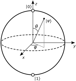
이러한 큐비트의 상태는 브로흐 구(Bloch sphere)에서 회전 나타낼 수 있다.
- 고전 동전(classical coin) : $$S(coin) = \frac{1}{2}|\text{H}\rangle + \frac{1}{2}|\text{T}\rangle$$
- 양자 동전(quantum coin) : $$|\psi\rangle = \frac{1}{\sqrt{2}}|0\rangle + \frac{1}{\sqrt{2}}|1\rangle$$
- 블로흐 구(Bloch sphere) : $$|\psi\rangle = \cos{\frac{\theta}{2}}|0\rangle + e^{i\phi}\sin{\frac{\theta}{2}}|1\rangle$$
이처럼 양자 동전은 측정 전에는 여러 상태가 동시에 존재하는 중첩 상태를 가지며, 측정을 통해서야 비로소 하나의 고전적인 상태로 붕괴한다.
아래는 rz gate를 통해서 0, 1이 각각 25%, 75%가 나오는 것을 확인할 수 있다.
from qiskit.circuit import QuantumCircuit
from qiskit.transpiler.preset_passmanagers import generate_preset_pass_manager
from qiskit.visualization import plot_histogram
import numpy as np
from qiskit_aer import AerSimulator
from qiskit.primitives import BackendSamplerV2 as Sampler
from qiskit.visualization import plot_bloch_multivector


backend = AerSimulator() # classical simulator
sampler = Sampler(backend=backend)

qcoin_phase = QuantumCircuit(1)
qcoin_phase.h(0)
# replace "x" below with a phase from 0 to 2*np.pi (this cell won't run if you leave x)
qcoin_phase.rz(np.pi*2/3, 0)
qcoin_phase.h(0)
plot_bloch_multivector(qcoin_phase)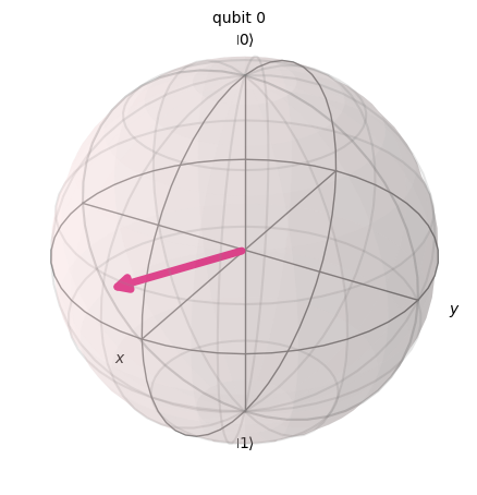
qcoin_phase.measure_all()


## Transpile

target = backend.target
pm = generate_preset_pass_manager(target=target, optimization_level=3)

qc_isa = pm.run(qcoin_phase)

## Execute

# On real hardware:

#pubs = [qc_isa]
#job = sampler.run(pubs, shots=1000)
#res = job.result()

#counts = res[0].data.meas.get_counts()

# or with Aer simulator with noise model from real backend
job = sampler.run([qc_isa], shots=1000)
counts=job.result()[0].data.meas.get_counts()

## Analyze
plot_histogram(counts)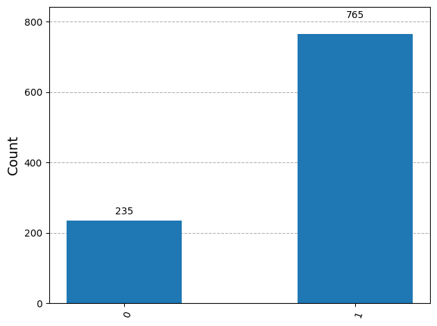
또한 블로흐 구는 다음과 같이 만들 수 있다. 여기서는 ry, rz gate를 통해서 회전을 표현하였다.
# Bloch sphere function
from qiskit.circuit import QuantumCircuit

def bloch_sphere(theta, phi):
    """
    Create a quantum circuit that prepares a qubit in a state defined by the polar angle theta and azimuthal angle phi.

    Args:
        theta (float): Polar angle in radians.
        phi (float): Azimuthal angle in radians.

    Returns:
        QuantumCircuit: A quantum circuit that prepares the specified state.
    """

    # Create a quantum circuit with one qubit
    qc = QuantumCircuit(1)

    # Apply RY gate to set the polar angle
    qc.ry(theta, 0)

    # Apply RZ gate to set the azimuthal angle
    qc.rz(phi, 0)

    return qc

bloch1 = bloch_sphere(2*np.arccos(np.sqrt(1/3)), np.pi/4)
plot_bloch_multivector(bloch1)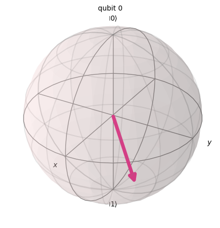
2. Measurement (측정)
앞서 살펴보았듯 양자 상태는 측정을 통해서 고전 상태로 확정이 된다. 양자컴퓨터에서 사용되는 qiskit에서는 양자 상태를 quantum resister(qubit)로 지정하고 연산을 진행하고 측정 결과를 classical resister에 값을 저장한다.
from qiskit.circuit import QuantumCircuit, Parameter
from qiskit.circuit import QuantumRegister, ClassicalRegister

theta = Parameter("$\\theta$")
phi = Parameter("$\\phi$")

# Define registers
qr = QuantumRegister(1, "q")
cr = ClassicalRegister(1, "c")
qc = QuantumCircuit(qr, cr)

# Add rotation gates for rotating the state of qubit 0 to random orientations
qc.rx(theta, 0)
qc.rz(phi, 0)
qc.measure(0, 0)

qc.draw("mpl")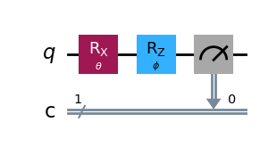
state, operator에 관하여
앞서 계속 0, 1 등의 상태(state)와 rx, ry 등의 gate(operator) 등을 사용하였는데, 대표적으로 자주 사용되는 state, operator를 정리해보면 좋을 것 같다.
state
다음은 양자 상태를 나타내는 나타내는 대표적인 basis이다. 브라켓(braket) notation을 주로 사용한다. 유클리드 크기(Euclidean norm, L2)를 사용하며 크기가 1인 벡터이다.
$$|0\rangle = \begin{bmatrix}1\\ 0\end{bmatrix}\text{,\quad\quad} |1\rangle = \begin{bmatrix}0\\ 1\end{bmatrix}$$
$$|+\rangle=\frac{1}{\sqrt{2}}(|0\rangle+i|1\rangle)\text{,\quad\quad}|-\rangle=\frac{1}{\sqrt{2}}(|0\rangle-|1\rangle)$$
$$|+i\rangle=\frac{1}{\sqrt{2}}(|0\rangle+|1\rangle)\text{,\quad\quad}|-i\rangle=\frac{1}{\sqrt{2}}(|0\rangle-i|1\rangle)$$
operator
양자회로에서의 연산은 측정(measure)을 제외하고는 기본적(이상적)으로는 유니타리(unitary) 연산이다. 유니타리 연산은 가역적이다. 다만, 현실에서는 noise와 주변(surround)과의 상호작용으로 완벽하게 가역적이지는 않다(비유니타리).
원인에는 결어긋남(decoherence), 위상 완화(dephasing), 게이트 오류(gate error) 등이 있다.
- decoherence : 환경과의 상호작용으로 양자상태가 빠르게 붕괴하는 현상. 이는 양자컴퓨터의 동작 시간을 제한하는 큰 요인이다.
- dephasing : decoherence의 일종으로 간섭을 이용하는 양자 상태가 외부 노이즈 등으로 위상(phase)을 잃어버리는 현상이다.
- gate error : gate를 통한 연산이 실제로는 오류가 존재하여 발생한다. 큐비트 하나에서 발생하는 single-qubit error와 두 큐비트에서 발생하는 two-qubit error가 있다. 이외에도 측정단계에서 이루어지는 readout error 등이 있다.
양자회로에서 사용하는 연산은 리 군(Lie group)에 속한다.
단일 큐비트 연산자 (Single-qubit Operators)
양자 연산은 유니타리 행렬 $U$에 의해 표현되며, 다음 조건을 만족한다.
$$U^{\dagger}U=UU^{\dagger}=I$$
- I (Identity) 게이트:
$$I = \begin{bmatrix}1&0\\ 0&1\end{bmatrix}$$
1. 파울리 게이트 (Pauli Gates)
가장 기본적인 유니타리 연산자이다. 또한 파울리 게이트는 에르미트(hermitian) 이기도 하여 $$H^{\dagger} = H$$이다. 따라서 임의의 파울리 게이트 $$\sigma$$는 $$\sigma^2=I$$이다.
- 파울리 X 게이트: 비트 플립(NOT) 연산을 수행합니다.
$$X = \begin{bmatrix}0&1\\ 1&0\end{bmatrix}$$ - 파울리 Y 게이트:
$$Y = \begin{bmatrix}0&-i\\ i&0\end{bmatrix}$$ - 파울리 Z 게이트: 위상 플립(Phase flip)을 수행합니다.
$$Z = \begin{bmatrix}1&0\\ 0&-1\end{bmatrix}$$
2. 하다마르 게이트 (Hadamard Gate)
큐비트를 균등 중첩 상태로 변환한다. $H|0\rangle = |+\rangle$ 이고, $H|1\rangle = |-\rangle$ 이다. $H^2=I$ 입니다.(hermitian)
$$H=\frac{1}{\sqrt{2}}\begin{bmatrix}1&1\\ 1&-1\end{bmatrix}$$
3. 위상 게이트 (Phase Gates)
다음과 같은 행렬로 표현되며, $|1\rangle$ 상태에만 위상을 변경한다.(정확히는 global phase는 무시가능하기 때문이다.)
$$P(\theta)=\begin{bmatrix}1&0\\ 0&e^{i\theta}\end{bmatrix}$$
- 주요 예시로는 $Z = P(\pi)$ 와 $S = P(\frac{\pi}{2})$ 가 있습니다.
4. 회전 게이트 (Rotation Gates)
블로흐 구면(Bloch sphere) 상에서 큐비트 상태를 회전시키는 유니타리 연산입니다.
- $$R_{x}(\theta)=\begin{bmatrix}cos(\frac{\theta}{2})&-isin(\frac{\theta}{2}) \\ -isin(\frac{\theta}{2})&cos(\frac{\theta}{2})\end{bmatrix}$$
- $$R_{y}(\theta)=\begin{bmatrix}cos(\frac{\theta}{2})&-sin(\frac{\theta}{2})\\ sin(\frac{\theta}{2})&cos(\frac{\theta}{2})\end{bmatrix}$$
- $$R_{z}(\theta)=\begin{bmatrix}e^{-i\theta/2}&0\\ 0&e^{i\theta/2}\end{bmatrix}$$
회전 게이트는 파울리 행렬을 지수 함수로 표현한 $R_{j}(\theta)=e^{i\frac{\theta}{2}\sigma_{j}}$ 형태로 정의될 수 있다. Talyor expansion을 가지고 확인이 가능하다.
5. 일반적인 유니타리 게이트
임의의 단일 큐비트 유니타리 연산은 세 개의 실수 매개변수 $\theta, \phi, \lambda$를 갖는 $U_3$ 게이트로 일반화될 수 있다.
$$U_{3}(\theta,\phi,\lambda)=\begin{bmatrix}cos(\frac{\theta}{2})&-e^{i\lambda}sin(\frac{\theta}{2})\ e^{i\phi}sin(\frac{\theta}{2})&e^{i(\phi+\lambda)}cos(\frac{\theta}{2})\end{bmatrix}$$
이 $U_3$ 게이트는 회전 게이트의 조합으로 해석될 수 있다.$$U_{3}(\theta,\phi,\lambda)=R_{z}(\phi)\cdot R_{y}(\theta)\cdot R_{z}(\lambda)$$
다중 큐비트 연산자 (Multi-qubit Operators)
- SWAP 게이트: 두 큐비트의 상태를 서로 교환하는 연산이다.
$$SWAP=\begin{bmatrix}1&0&0&0\\ 0&0&1&0\\ 0&1&0&0\\ 0&0&0&1\end{bmatrix}$$ - CNOT 게이트 (CX): 제어 큐비트가 $|1\rangle$일 때 대상 큐비트에 X 연산을 적용합니다.
$$CNOT=\begin{bmatrix}1&0&0&0\\ 0&1&0&0\\ 0&0&0&1\\ 0&0&1&0\\end{bmatrix}$$ - CZ 게이트: 제어 큐비트가 $|1\rangle$일 때 대상 큐비트에 Z 연산을 적용합니다.
$$CZ=\begin{bmatrix}1&0&0&0\\ 0&1&0&0\\ 0&0&1&0\\ 0&0&0&-1\end{bmatrix}$$
3. Uncertainty (불확정성)
불확정성 원리(uncertainty principle)는 다음과 같다.
$$\Delta x \Delta p \geq \frac{\hbar}{2}$$
여기서 $$\Delta$$가 uncertainty에 해당하는 것으로 표준편차의 개념이다. 따라서 다음과 같이 계산을 할 수 있다.
$$(\Delta S)^2 = \left<(S- \left<S\right>)^2\right>= \left<S^2 \right> - \left<S\right>^2$$
하이젠베르크의 불확정성 원리를 일반화하면 두 operator A, B에 대해 다음과 같이 나타난다.(Cauchy–Schwarz inequality 이용)
$$\Delta A \Delta B \geq \frac{1}{2}|\left<[A, B]\right>|$$
여기서 파울리 연산은 $$\sigma_i\sigma_j = i\sigma_k$$이므로 $$\Delta \sigma_i \Delta \sigma_j \geq \frac{1}{2}|\left<\sigma_k\right>|$$ 와 같이 나타난다.
# Step 1: Map the problem into a quantum circuit

from qiskit.circuit import Parameter
import numpy as np
from qiskit.circuit import QuantumCircuit, QuantumRegister, ClassicalRegister
from qiskit.quantum_info import SparsePauliOp
from qiskit.transpiler.preset_passmanagers import generate_preset_pass_manager

from qiskit_ibm_runtime import (
    Batch,
    SamplerV2 as Sampler,
    EstimatorV2 as Estimator
)

from qiskit_aer import AerSimulator

backend = AerSimulator()  # classical simulator

# Specify observables
obs1 = SparsePauliOp("X")
obs2 = SparsePauliOp("Y")
obs3 = SparsePauliOp("Z")

# Define registers
qr = QuantumRegister(1, "q")
cr = ClassicalRegister(1, "c")
qc = QuantumCircuit(qr, cr)

# Rotate away from |0>
theta = Parameter("θ")
qc.ry(theta, 0)

params = np.linspace(0, 2, num=21)

# Step 2: Transpile the circuit

pm = generate_preset_pass_manager(backend=backend, optimization_level=3)
qc_isa = pm.run(qc)
obs1_isa = obs1.apply_layout(layout=qc_isa.layout)
obs2_isa = obs2.apply_layout(layout=qc_isa.layout)
obs3_isa = obs3.apply_layout(layout=qc_isa.layout)

# Step 3: Run the circuit simulation

with Batch(backend=backend) as batch:
    estimator = Estimator(mode=batch)
    pubs = [(qc_isa, [[obs1_isa], [obs2_isa], [obs3_isa]], [params])]
    job = estimator.run(pubs, precision=0.01)
    res = job.result()

    #batch.close()

# Step 4: Post-processing and classical analysis.
xs = res[0].data.evs[0]
ys = abs(res[0].data.evs[1])
zs = res[0].data.evs[2]

# Calculate uncertainties

delx = []
delz = []
prodxz = []
for i in range(len(xs)):
    delx.append(abs((1 - xs[i] * xs[i])) ** 0.5)
    delz.append(abs((1 - zs[i] * zs[i])) ** 0.5)
    prodxz.append(delx[i] * delz[i])

# Here we can plot the results from this simulation.
import matplotlib.pyplot as plt

plt.plot(params, delx, label=r"$\Delta$ X")
plt.plot(params, ys, label=r"$\langle$ Y $\rangle$")
plt.plot(params, delz, label=r"$\Delta$ Z")
plt.plot(params, prodxz, label=r"$\Delta$X $\Delta$Z")
plt.xlabel(r"$\theta$")
plt.ylabel("Expectation/Uncertainty Values")
plt.legend()
plt.show()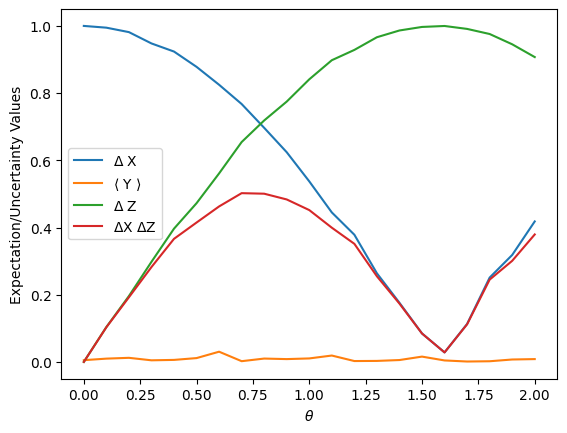
4. Entanglement (얽힘)
아인슈타인(Einstein)은 양자 상태의 결과가 본질적으로 미리 결정되어 있다고 주장한다. 측정의 결과는 우리가 알지 못하더라도, 이미 자연에 의해 정해져 있다는 것이다. 이는 때때로 '숨은 변수(hidden variables)'라고 불리는데, 이는 다른 축을 따라 투영된 값들이 미리 정해져 있지만 우리에게는 숨겨져 있기 때문이라는 것이다.
- 측정은 큐비트의 상태를 만드는 것이 아니라, 미리 존재하던 상태를 드러내는 역할만 한다.
- 전자와 양전자의 스핀 사이에는 인과적 영향이 없습니다. 두 입자 사이의 상관관계는 각운동량 보존이라는 초기 조건에 의해 발생한다.
보른(Born) 관점은 양자 상태가 측정되기 전까지는 실제로 '미결정(undetermined)' 상태이며 물리적으로 제대로 정의되지 않는다고 주장한다.
- 스핀을 측정하면 모든 가능성의 공간이 단일하고 확정된 상태로 '붕괴(collapses)'한다.
- 한 입자(양전자)의 스핀을 측정하면, 거리에 상관없이 다른 입자(전자)의 스핀도 정확히 반대 방향으로 확정되도록 강제한다. 이 효과를 '원격 유령 작용(spooky action at a distance)' 또는 '비국소 물리학(non-local physics)'이라고 부른다.
즉, 아인슈타인의 관점에서는 숨은 변수에 의해서 $$|S| \leq 2$$라는 부등식을 만족한다고 보았지만, 양자 얽힘을 이용한 보른의 관점에서는 $$|S| \leq 2\sqrt2$$라는 것을 확인할 수 있었고, 이는 벨 상태(Bell state)일 때 가능하다는 것을 알 수 있었다.
CHSH inequality
CHSH 게임은 국소적 숨은 변수(local hidden variables) 이론(고전적 관점)이 양자역학을 완벽히 설명할 수 있는지 실험적으로 검증하기 위해 고안된 게임이다.
게임의 규칙
이 게임에는 두 명의 참가자, Alice와 Bob이 있다. 이들은 서로 소통할 수 없다.
- 심판이 Alice에게 무작위 비트 $x \in {0, 1}$를, Bob에게 무작위 비트 $y \in {0, 1}$를 각각 전달한다.
- Alice는 $x$를 받고 비트 $a \in {0, 1}$를 출력한다.
- Bob은 $y$를 받고 비트 $b \in {0, 1}$를 출력한다.
- 두 사람은 자신의 출력 $a$와 $b$가 $a \oplus b = x \cdot y$라는 승리 조건을 만족하면 승리한다.
($x \cdot y$는 AND 연산, $\oplus$는 XOR 연산)
승리 조건은 네 가지 입력 조합에 대해 다음과 같습니다.
- $x=0, y=0 \implies a \oplus b = 0$ (a와 b는 같아야 함)
- $x=0, y=1 \implies a \oplus b = 0$ (a와 b는 같아야 함)
- $x=1, y=0 \implies a \oplus b = 0$ (a와 b는 같아야 함)
- $x=1, y=1 \implies a \oplus b = 1$ (a와 b는 달라야 함)
고전적 전략 (국소적 숨은 변수 관점)
고전적 관점에서는 Alice와 Bob이 미리 정해진 전략을 따르지만, 입력 $x, y$를 받은 후에는 소통할 수 없다. 따라서 그들은 어떤 상황에서든 입력 $x,y$와 관계없이 항상 같은 출력(예: $a=0, b=0$)을 내거나, 항상 다른 출력(예: $a=0, b=1$)을 내는 등 정해진 규칙에 따라 행동할 수밖에 없다.
최선의 고전적 전략은 네 가지 경우 중 세 가지를 맞히는 것입니다. 예를 들어, 항상 같은 출력만 내기로 약속하면 $x=1, y=1$인 경우를 제외하고는 모두 승리한다. 이 경우 승리 확률은 $3/4$ (75%)이다. 따라서 고전적 승리 확률의 최댓값은 75%입니다.
양자적 전략 (벨 상태 이용 관점)
양자역학적 관점에서는 Alice와 Bob이 게임 시작 전에 얽힘 상태(entangled state)를 공유합니다. 이전에 논의된 것처럼, 얽힘 상태는 국소적인 정보만으로는 설명할 수 없는 비국소적(non-local) 상관관계를 가집니다. 대표적인 얽힘 상태인 벨 상태($|\psi^{+}\rangle=\frac{1}{\sqrt{2}}(|01\rangle+|10\rangle)$)를 공유하는 것이 최적의 전략입니다.
- 게임 시작 전, Alice와 Bob은 얽힌 큐비트를 각각 하나씩 가진다. Alice는 큐비트 0, Bob은 큐비트 1을 갖는다.
- 입력 $x$를 받은 Alice는 x=0이면 z축, x=1이면 x축을 측정한다.
- 입력 $y$를 받은 Bob은 y=0이면 $$\pi/4$$, y=1이면 $$-\pi/4$$
- 각각 측정한 결과를 a, b로 선택한다.
이러한 양자 전략을 사용했을 때의 최대 승리 확률은 약 85.3%=$$\cos^2(\frac{\pi}{8})$$ 입니다. 이는 고전적 전략의 최댓값인 75%를 초과하는 값입니다.
결론
CHSH 게임은 양자 얽힘이 국소적 숨은 변수 이론만으로는 설명할 수 없는 비국소적 상관관계를 실제로 제공한다는 것을 보여준다. 이 게임은 양자역학의 예측이 고전 물리학의 예측을 뛰어넘는다는 것을 증명하는 가장 강력한 실험적 증거 중 하나이다.
구현
from qiskit import QuantumCircuit
import numpy as np

def create_chsh_circuit(x, y):
    """Builds Qiskit circuit for Alice & Bob's quantum strategy."""
    qc = QuantumCircuit(2, 2, name=f'CHSH_{x}{y}')

    # bell state
    qc.h(0)
    qc.cx(0, 1)
    qc.barrier()

    # Alice
    if x == 1:
        qc.h(0) # H 게이트를 가해 X 방향으로 회전


    # Bob
    if y == 1:
        qc.ry(np.pi/4, 1)
    elif y == 0:
        qc.ry(-np.pi/4, 1)
    qc.barrier()


    qc.measure([0, 1], [0, 1]) # q0 -> c0 (앨리스), q1 -> c1 (밥) // 'ba' 순서로 표시됨

    return qc

circuits = []
input_pairs = []
for x_in in [0, 1]:
    for y_in in [0, 1]:
        input_pairs.append((x_in, y_in))
        circuits.append(create_chsh_circuit(x_in, y_in))

print("Quantum circuit for inputs x=1, y=1 (Check your Exercises 1 & 2 implementation):")
if len(circuits) == 4:
    display(circuits[3].draw('mpl')) # (x,y) = (1,1)
else:
    print("Circuits not generated. Run previous cell after completing Exercises 1 & 2.")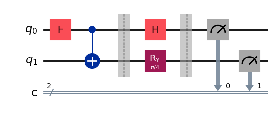
from qiskit_aer import AerSimulator
from qiskit.transpiler import generate_preset_pass_manager
from qiskit_ibm_runtime import SamplerV2 as Sampler
from qiskit.visualization import plot_histogram

backend = AerSimulator()
pm = generate_preset_pass_manager(backend=backend, optimization_level=1)

SHOTS = 1024

print("Preparing circuits for the simulator...")
isa_qc_chsh = pm.run(circuits)

sampler_chsh = Sampler(mode=backend) # SamplerV2
job_chsh = sampler_chsh.run(isa_qc_chsh, shots=SHOTS)
results_chsh = job_chsh.result()

# SamplerV2: 고전 레지스터의 이름 기본값이 'c'일 때 results_chsh[i].data.c.get_counts()
counts_list = [results_chsh[i].data.c.get_counts() for i in range(len(circuits))]

print("\n--- Simulation Results (Counts) ---")
for i, (x, y) in enumerate(input_pairs):
    print(f"Inputs (x={x}, y={y}):")
    sorted_counts = dict(sorted(counts_list[i].items()))
    print(f"  Outcomes (ba): {sorted_counts}")

print("\nPlotting results...")
display(plot_histogram(counts_list,
                       legend=[f'(x={x}, y={y})' for x, y in input_pairs],
                       title='CHSH Game Outcomes (ba format)'))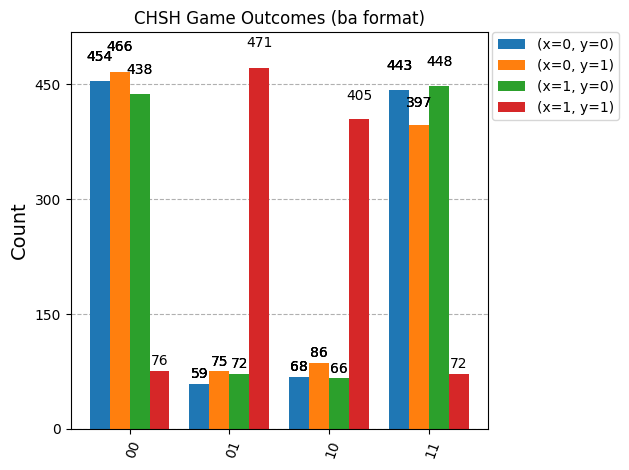
win_probabilities = {}
print("--- Calculating Win Probabilities ---")

for i, (x, y) in enumerate(input_pairs):
    counts = counts_list[i]

    target_xor_result = 0
    wins_for_this_case = 0
    sorted_counts = dict(sorted(counts_list[i].items()))
    if (x, y) == ((0, 0) or (0, 1) or (1, 0)):
        wins_for_this_case += sorted_counts['00']
        wins_for_this_case += sorted_counts['11']
    elif (x, y) == (0, 1):
        wins_for_this_case += sorted_counts['00']
        wins_for_this_case += sorted_counts['11']
    elif (x, y) == (1, 0):
        wins_for_this_case += sorted_counts['00']
        wins_for_this_case += sorted_counts['11']
    elif (x, y) == (1, 1):
        target_xor_result += sorted_counts['01']
        target_xor_result += sorted_counts['10']
        wins_for_this_case += sorted_counts['01']
        wins_for_this_case += sorted_counts['10']


    prob = wins_for_this_case / SHOTS if SHOTS > 0 else 0
    win_probabilities[(x, y)] = prob
    print(f"Inputs (x={x}, y={y}): Target (a XOR b) = {target_xor_result}. Win Probability = {prob:.4f}")

avg_win_prob = sum(win_probabilities.values()) / 4.0
P_win_quantum_theory = np.cos(np.pi / 8)**2  # ~0.8536
P_win_classical_limit = 0.75

print("\n--- Overall Performance ---")
print(f"Experimental Average Win Probability: {avg_win_prob:.4f}")
print(f"Theoretical Quantum Win Probability: {P_win_quantum_theory:.4f}")
print(f"Classical Limit Win Probability:     {P_win_classical_limit:.4f}")

if avg_win_prob > P_win_classical_limit + 0.01: # 시뮬레이션이므로 오차 허용
    print(f"\nSuccess! Your result ({avg_win_prob:.4f}) clearly beats the classical 75% limit!")
    print(f"It's likely close to the theoretical quantum prediction of {P_win_quantum_theory:.4f}.")
elif avg_win_prob > P_win_classical_limit - 0.02 : # 약간의 에러
     print(f"\nClose, but no cigar? Your result ({avg_win_prob:.4f}) is around the classical limit ({P_win_classical_limit:.4f}).")
     print("Check your solutions for Exercises 1-4 carefully, especially the win counting logic in Ex 4.")
else:
    print(f"\nHmm, the result ({avg_win_prob:.4f}) is unexpectedly low, even below the classical limit.")
    print("There might be an error in Exercises 1-4. Please review your circuit and analysis code.")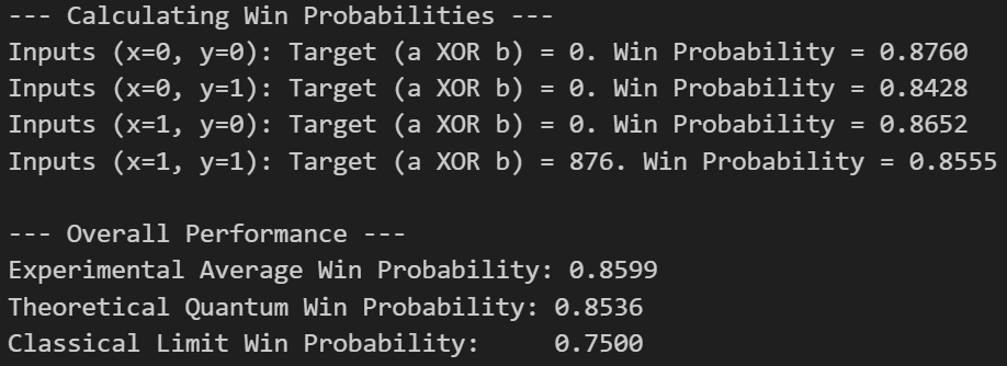
출처
- Quantum Mechanics: Superposition with Qiskit
- Quantum Mechanics: The Stern-Gerlach experiment using quantum computers
- Quantum Mechanics: Exploring uncertainty
- Quantum Mechanics: The nature of quantum states: hidden variables versus Bell's inequality
- wikipedia: bloch sphere
- wikipedia: Lie group
- wikipedia: CHSH inequality
- Basics of quantum information
'양자컴퓨터' 카테고리의 다른 글
| Computer Science for Quantum Computing (0) | 2025.11.01 |
|---|---|
| 양자 컴퓨팅 구현을 위한 조건: DiVincenzo's Criteria (0) | 2025.11.01 |
| 2025-1 QIYA (Quantum Informatics at Yonsei Academy) IBM Learning Course Team Project (0) | 2025.10.31 |